
[Basic Theory.1] Basic Theory
Energy Units and Molecular Spectra
Plane Polarized electromagetic radiation
[Figure. 1] illustrates a wave of polarized electromagnetic radiation traveling in the x-direction. The electric component is y-direction and magnetic is z-direction.
Hereafter, we consider only the former. (Don’t involve magnetic phenomena). The electric field strength (E) at a given time (t) is expressed by
\(E_0\) is the amplitude, \(\nu\) is the frequency of radiation.
The distance between two points of the same phase in successive waves is called the “wavelength” , \(\lambda\), which us measured in units.(\(\mathring{A}\)(angstrom), \(nm\)(nanometer), \(m\mu\)(millimicron), and \(cm\)(centimeter)). The relationships between them are:
Frequency
The frequency, \(\nu\) is the number of waves in the distance light travels in one second. Thus,
\[\nu = \frac{c}{\lambda} \tag{3}\]\(c\) is the velocity of light \((3 \times 10^{10} cm/s)\). And if \(\lambda\) is in the unit of centimeters, its dimension is \((cm/s)/(cm) = 1/s\). This “reciporal second” unit is also called the “hertz” \((Hz)\). There’s another parameter is the “wavenumber”, \(\tilde{\nu}\) defined by
\[\tilde{\nu} = \frac{\nu}{c} \tag{4}\]The difference between \(\nu\) and \(\tilde{\nu}\) is obvious. It has the dimension of \((1/s)/(cm/s) = 1/cm.\) By combining Eq.(3),Eq.(4) we have
\[\tilde{\nu} = \frac{\nu}{c} = \frac{1}{\lambda}(cm^{-1}) \tag{5}\]Also, we can express by \(v\)
\[\nu = \frac{c}{\lambda} = c \tilde{\nu} \tag{6}\]As shown earlier, the wavenumber\((\tilde{\nu})\) and frequency \((\nu)\) are different parameters, yet these two terms are often used interchangeably. Thus, we can express by IR and Raman spectrosopists such as “frequency shift of \(10 \;cm^{-1}\)”.
Interacts with an electromagetic field
We can know a transfer energy from the field to the molecule and it can occur only when Bohr’s frequency condition is satisfied.(If a molecule interacts with an electromagetic field).
\[\Delta E = h\nu = h\frac{c}{\lambda} = hc\tilde{\nu} \tag{7}\]Here \(h\) is Planck’s constant \((6.62 \times 10^{-27}erg\; s)\) and \(\Delta E\) is the difference in energy between two quantized states. Thus, \(\tilde{v}\) is directly proportional to the energy of transition.
Let’s Suppose that
\[\Delta E = E_2 - E_1 \tag{8}\]\(E_2\) : Energy of the exicted states, \(E_1\) : Energy of the gound states.
Then, the molecule absorbs \(\Delta E\) when it is exited from \(E_1\) to \(E_2\) ( \(E_1 \rightarrow E_2\) ) and emits \(\Delta E\) when it reverts from \(E_2\) to \(E_1\) ( \(E_2 \rightarrow E_1\) ).
We can express \(\Delta E\) in terms of various energy units. Thus, \(1 cm^{-1}\) is :
\[\begin{align} \Delta E &= E^2 - E^1 = hc\tilde{\nu} \\ &=[6.62 \times 10^{-27} (erg \; s)][3 \times 10^{10} (cm/s)][1(1/cm)] \\&= 1.99 \times 10^{-16} &\; (erg/molecule) \\ &= 1.99 \times 10^{-23} &\; (joule/molecule)\\ &= 2.86 &\; (cal/mole) \\ &=1.24 \times 10^{-4} &\; (eV/molecule) \end{align}\]Observed Region
We mainly concern with vibrational transitions which are observed in infrared(IR) or Raman Spectra. They appear in the \(10^{-4} \sim 10^2 \; (cm^{-1}) \;\) region and originate from vibrations of nuclei constituting the molecule. Raman spectra are related to electronic transitions. Thus, it is important to know the relationship between electronic and vibrational states.

Furthermore, vibrational spectra of small molecules in the gaseous state exhibit rotational fine structures. Thus, it’s also important to know the relationship between vibrational and rotational states. [Figure. 3]

Vibration of a Diatomic Molecule
Classical treatment
Consider the vibartion of a diatomic molucule in which two atoms are connected by a chemical bond.[Figure. 4]

Each masses of atom 1 and 2 are \(m_1\) and \(m_2\) and \(r_1\) and \(r_2\) are the distances from the center of gravity (C.G.) to the atoms designated. Thus, \(r_1 + r_2\) is the equilibrium distance. Then, the conservation requires the ralationships:
Eq.9 and Eq.10 combine
\[x_1 = \Big(\frac{m_2}{m_1}\Big)x_2 \quad \text{or} \quad x_2=\Big(\frac{m_1}{m_2}\Big)x_1 \tag{11}\]In the classical treatment, we can regard the chemical bond as a spring. It obeys the Hooke’s law, so we can express the restoring force, \(f\) :
\[f = -K(x_1 + x_2) \tag{12}\]Where K is the force constant, and the directions of the force are opposite to each other. Now, combining the Eq.11 and Eq.12, we obtain :
\[f = -K \Big(\frac{m_1 + m_2}{m_1}\Big) = -K \Big(\frac{m_1 + m_2}{m_2}\Big) \tag {13}\]Using Newton’s equation of motion, we obtain for each atom as :
\[\begin{align} m_1\frac{d^2 x_1}{dt^2} = -K \Big(\frac{m_1 + m_2}{m_2}\Big)x1 \\ m_2\frac{d^2 x_2}{dt^2} = -K \Big(\frac{m_1 + m_2}{m_2}\Big)x2 \tag{14} \end{align}\]Multiply for each atom \(\Big(\frac{m_2}{m_1 + m_2} \Big)\) and adding, we obtain :
\[\frac{m_1 m_2}{m_1 + m_2} \Big(\frac{d^2 x_1}{dt^2} + \frac{d^2 x_2}{dt^2}\Big) = -K(x_1 + x_2) \tag{15}\]Introducing the reduced mass \((\mu)\) and the displacement \((q = x_1 + x_2)\), the Eq.15 is written as :
\[\mu \frac{d^2 q}{dt^2} = -Kq \tag{16}\]Here, the solution of thie differential equation is
\[q=q_0 sin(2\pi \nu_0 t + \varphi) \tag{17}\]where \(q_0\) is the maximum displacement and \(\varphi\) is the phase constant.(depends on the inital conditions.) \(v_0\) is the classical vibrational frequency given by
\[\nu_0 = \frac{1}{2\pi} \sqrt{\frac{K}{\mu}} \tag{18}\]We can calculate the potential energy \((V)\) and the kinetic energy \((T)\) as :
\[\begin{align*} dV &= -f\;dq = Kq\;dq \\ V &= \frac{1}{2}Kq^2 \\ &=\frac{1}{2} Kq^2_0 sin^2(2\pi \nu_0 t + \varphi) \\ &=2\pi^2 \nu_0^2 \mu q^2_0 sin^2(2\pi\nu_0 t + \varphi) \tag{19}\\ \\ T &= \frac{1}{2} m_1 \Big(\frac{dx_1}{dt}\Big)^2 + \frac{1}{2} m_2 \Big(\frac{dx_2}{dt} \Big)^2 \\ &= \frac{1}{2}\mu \Big(\frac{dq}{dt}\Big)^2 \\ &= 2\pi^2 \nu^2_0 \mu q_0^2 cos^2(2\pi \nu_0 t + \varphi) \tag{20} \end{align*}\]Thus, the total energy \((E)\) is :
\[\begin{align*} E &= T + V \\ &=2\pi^2\nu^2_0q_0^2 \quad (\because sin^2 x + cos^2 x = 1) \\ &= constant \tag{21} \end{align*}\]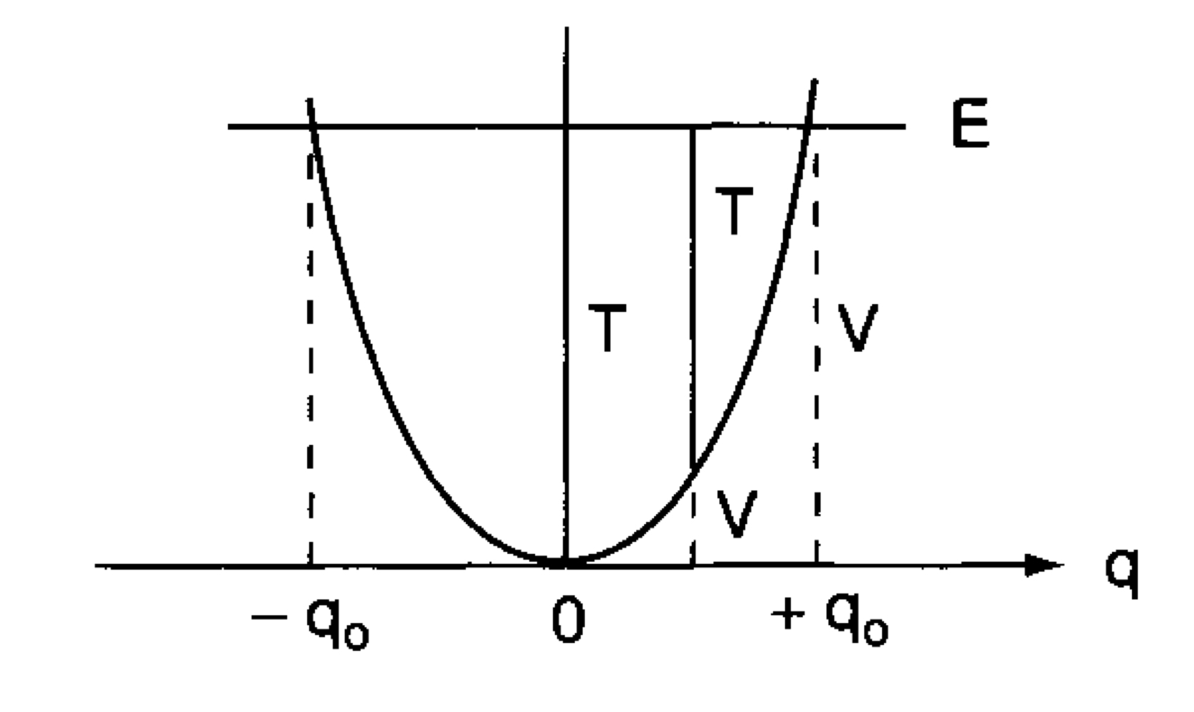
[Figure. 5] is based on the book. It shows the plot of \(V\) as a function of \(q\) and looks like a vibrator called a harmonic oscillator.
Quantum Mechanics
Considering a motion of a single particle having mass \(\mu\), the vibration can be written for the Schrödinger equation as
\[\frac{d^2 \psi}{dq^2} + \frac{8 \pi^2 \mu }{h^2} \Big(E-\frac{1}{2}Kq^2 \Big)\psi = 0 \tag{22}\]If the \(\psi\) must be single-valued,finite and continuous, the eigenvalues are written as by solving the Eq.22 :
\[E_v = h\nu \Big(v + \frac{1}{2} \Big) = hc\tilde{\nu} \Big( v + \frac{1}{2}\Big) \tag{23}\]And the frequency of vibration is as follows seems like Eq.18
\[\nu = \frac{1}{2\pi} \sqrt{\frac{K}{\mu}} \tag{24}\]where \(v\) is the vibrational quantum number, and having the values 0,1,2… So, the corresponding eigenfunctions are :
\[\psi _v = \frac{(\alpha / \pi)^{1/4}}{\sqrt{2^{\mathrm{v}} v!}}e^{-\alpha q^2 / 2} H_v(\sqrt{\alpha q}) \tag{25}\]where \(\alpha = 2\pi \sqrt{\mu K/h} = 4\pi^2 \mu v/h\) and \(H_v(\sqrt{\alpha q})\) is a Hermite polynomial of the $\mathrm{v}^{th} $ degree.
Thus, the eigenvalues and the corresponding eigenfunctions are
\[\begin{align*} &v = 0, \quad E_0 = \frac{1}{2} hv, \quad \psi _0 = (\alpha / \pi)^{1/4} e^{-\alpha q^2 /2} \\ &v = 1, \quad E_1 = \frac{3}{2} hv, \quad \psi _1 = (\alpha / \pi)^{1/4} 2^{1/2}qe^{-\alpha q^2 /2} \tag{26} \end{align*}\] \[\vdots\]Difference of the frequency between classical & quantum-mechanical
The quantum mechanical frequency(Eq.24) is same as the classical frequency(Eq.18). However, there are some differences noted between the two treatments.
First, the zero-state Engergy. Classicaly, the energy E is zero when q is zero.
\[q=0 \rightarrow E=0 \tag{27-1}\]But, in the Quantum-mechanically, the lowest E state \((v=0)\) has the energy, \(\frac{1}{2} h\nu\) (=zero point energy). That’s because the Heisenberg’s uncertainly prinicple.
\[v=0 \rightarrow E = \frac{1}{2} h\nu \quad (\because uncertainly principle) \tag{27-2}\]Second, continuity of a vibrator. Classicaly, vibrator can change contiuosly. But In quantum mechanics, the energy, E can change only in units of \(h\nu\).
| Vibrator | Continuity |
|---|---|
| Classical | continuous |
| Quantum | units of $h\nu$ |
Thirdly, probability of breakaway from the parabola. Classically, the vibration is confined within the parabola. Because if $\vert q \vert > \vert q_0 \vert$, the T becomes negative. Contrary, in quantum-mechanics, the probability (of finding q outside the parabola) is not zero since the tunnel effect.
Hot Band

Hereafter, talk about the separation between the two vibrational levels.
In the case of a harmonic oscillator, that is always same with $h\nu$. But an actual molecule is not the case. The potential is approximated by the Morse potential function shown by the solid curve like [Figure. 6].
where $D_e$ is the dissociation energy, $\beta$ is a measure of the curvature an the bottom of the potentail well.
The eigenvalues by solving with the Schrödinger equation :
where $w_e$ is the wavenumber corrected for anharmonicity, $\chi_e w_e$ indicates the magnitude of anharmonicity.
By Eq.29, the E levels of the anharmonic oscillator are no longer equidistant. And the separtion decreases with increasing $\nu$ like [Figure. 6].
According to quantum-mechanics, Only in a harmonic oscillator, those transitions involving $\Delta v = \pm 1 $ are allowed. Else, the transitions involving $\Delta v = \pm 2, \pm 3, \dots$ (overtones). Both in IR and Raman spectra, many $\Delta v = \pm 1 $ transitions that of $v = 0 \leftrightarrow 1 $ appears most strongly. That is expected from the Maxwell-Boltzmann distribution law, which states that the population ration of the $v=1 $ and $v = 0$ states is given by
where $\Delta E$ is the energy difference between the two states, $k$ is Boltzmann’s constant $(1.3807 \times 10^{-16} \; erg/degree)$, and $T$ is the absolute temperature. Since $\Delta E = hc\tilde{v}$, the ratio is inversely proportional with $\tilde{v}$. $(\frac{P_{v=1}}{P_{v=0}} \propto \frac{1}{\tilde{v}}) $
Example, the $\tilde{v}$ of $\mathrm{H}_2$ is $4,160 \; cm^{-1}$, $T$ is room temperature $(300K)$
\[\begin{align*} kT &= 1.38 \times 10^{-6} \; (erg/degree) \quad 300 \; (degree) \\ &= [4.14 \times 10^{-14} \; (erg)] / [1.99 \times 10^{-16} \; (erg)(cm^{-1})] \\ &= 208 \; (cm^{-1}) \tag{31} \\ \end{align*}\]Then, the ratio is
\[\frac{P_{v=1}}{P_{v=0}}=e^{-hc(4,160)/208} = 2.19 \times 10^{-9} \tag{32}\]That means almost all of the molecules are at $v=0$.
If $\tilde{v} = 213 \; cm^{-1} $ ( $I_2$ molecule), the ratio is 0.36. That is abpit 27% of the $I_2$ molecules are at $v=1$ state. In this case, the transition $ v = 1 \rightarrow 2 $ should be observed on the low-frequency side of the fundamental with much less intensity. Such a transition is called a “hot band” since it tends to appear at higher temperatures.
Origin of Raman Spectra
IR absorption
Now measure the absorption of IR by the sample as a function of frequency. The molecule absorbs $\Delta E = hv$ from the IR source at each vibrational transition. The intensity of IR absorption is governed by the Beer-Lambert Law :
\[I = I_0 e^{-\varepsilon c d} \tag{33}\]In IR spectroscopy, it’s customary to plot the percentage transmission $(T)$ versus wave number $(\tilde{\nu})$:
\[T(\%) = \frac{I}{I_0} \times 100 \tag{34}\]Note : $T(\%)$ is not proportional to $c$.
For quntitative analysis, the absorbance $(A)$ defined here should be used:
Raman spectra
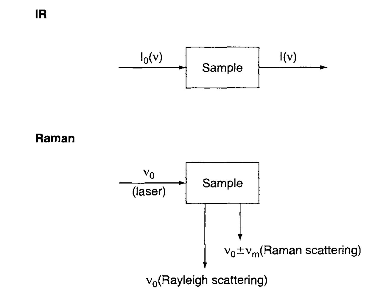
In [Figure. 7], Raman spectra is different from that of IR spectra. The scattered light from the sample is observed in the direction perpendicualr to the incident beam. That consists of two types :
- Rayleigh scattering : is strong and has the same frequency as the incident beam.
- Raman scattering : is very weak ( $ ~ 10^{-5} $ of the incident beam) and has frequencies $ \nu_0 \pm \nu_m$
At the Raman scattering, $\nu_0 - \nu_m$ is Stokes, and $\nu_0 + \nu_m$ is anti-Stokes lines. Thus, we measure the vibrational frequncy $(\nu_m)$ as a shift from the incident beam frequncy $(\nu_0)$.
In classical theory, Raman scattering follows:
If a diatomic molecule is irradiated, an electric dipole moment P is induced :
\[P = \alpha E = \alpha E_0 cos 2\pi \nu_0 t \tag{37}\]The $\alpha$ is a proportionally constant ( polarizability). Frequency of the vibrating molecule is $\nu_m$, $q_0$ is the vibrational amplitude, the nuclear displacement q:
\[q = q_0 cos 2\pi \nu_m t \tag{38}\]For a small amplitude of vibration, $\alpha$ is a linear function of q. Thus, we can write
\[\alpha = \alpha_0 + \Big(\frac{\partial \alpha}{\partial q} \Big)_0 q_0 + \cdots \tag{39}\]Combining Eq.37 & Eq.38, we obtain :
\[\begin{align} \\ P &= \alpha E_0 cos 2\pi \nu_0 t \\ &= \alpha_0 e_0 cos 2\pi \nu_0 t + \Big(\frac{\partial \alpha}{\partial q}\Big)_0 q E_0 cos 2\pi \nu_0 t \\ &= \alpha_0 E_0 cos 2\pi \nu_0 t + \Big(\frac{\partial \alpha}{\partial q}\Big)_0 q_0 E_0 cos2\pi \nu_0 t cos 2\pi \nu_m t \\ &= \alpha_0 E_0 cos 2\pi \nu_0 t + \frac{1}{2} \Big(\frac{\partial \alpha}{\partial q})_0 q_0 E_0 [cos {2\pi(\nu_0 + \nu_m)t} + cos {2\pi (\nu_0 - \nu_m)t}] \tag{39} \\ \end{align}\]
Leave a comment